Solving First-Order ODEs

Teng-Jui Lin

Content adapted from UW AMATH 301, Beginning Scientific Computing, in Spring 2020.

• Solving first-order ODEs

  • Methods

    • Forward Euler

    • Backward Euler

    • Midpoint method

    • Fourth-order Runge-Kutta (RK4) method

  • Error

• scipy implementation

  • Solving first-order ODEs by scipy.integrate.solve_ivp()

Solving first-order ODEs

Suppose we have an ODE of the form

$$\dot{y}=f(t,y).$$

Forward Euler

Forward Euler uses the forward difference as approximation for the derivative, having formula of

$$y_{k+1}=y_k+f(y_k,t_k)\mathrm{\Delta }t$$

Backward Euler

Backward Euler uses backward difference to approximate the derivative, having implicit formula of

$$y_{k+1}=y_k+f(y_{k+1},t_{k+1})\mathrm{\Delta }t$$

At each step of backward Euler, $y_{k+1}$ can be found by finding the root of

$$y_k+f(y_{k+1},t_{k+1})\mathrm{\Delta }t-y_{k+1}=0$$

where $y_k$ is known.

Midpoint method

Midpoint method uses the slope at the midpoint as approximation for the derivative:

1. Do a half step of forward Euler using the slope at starting point $k_1$, record the slope at midpoint $k_2$

2. Use the slope at the midpoint $k_2$ to do a full step of forward Euler to find $y_{k+1}$

The method follows the steps

$$\begin{array}{r}\begin{array}{rl}{k}_1& =f(y_k)\\ k_2& =f(y_k+{\displaystyle \frac{\mathrm{\Delta }t}{2}}{k}_1)\\ y_{k+1}& =y_k+k_2\mathrm{\Delta }t\end{array}\end{array}$$

Fourth-order Runge-Kutta (RK4)

Fourth-order Runge-Kutta method uses a weighted average of slopes at the midpoint and endpoint as approximation for the derivative:

1. Do a half step of forward Euler using the slope at starting point $k_1$, record the slope at midpoint $k_2$

2. Use the slope at midpoint $k_2$ to do another half step of forward Euler, record the new slope at midpoint $k_3$

3. Use the new slope at midpoint $k_3$ to do a full step of forward Euler, record the slope at the endpoint $k_4$

4. Use a weighted average of all slopes $k_1,k_2,k_3,k_4$ to find $y_{k+1}$

The method follows the steps

$$\begin{array}{r}\begin{array}{rl}{k}_1& =f(y_k)\\ k_2& =f(y_k+k_1{\displaystyle \frac{\mathrm{\Delta }t}{2}})\\ k_3& =f(y_k+k_2{\displaystyle \frac{\mathrm{\Delta }t}{2}})\\ k_4& =f(y_k+k_3\mathrm{\Delta }t)\\ y_{k+1}& =y_k+{\displaystyle \frac{\mathrm{\Delta }t}{6}}(k_1+2k_2+2k_3+k_4)\end{array}\end{array}$$

Errors of methods

The order of errors of each method is shown below:

Method	Order	Global Error	Local Error	Explicit/Implicit
Forward Euler	1	$\mathcal{O}(\mathrm{\Delta }t)$	$\mathcal{O}(\mathrm{\Delta }{t}^2)$	Explicit
Backward Euler	1	$\mathcal{O}(\mathrm{\Delta }t)$	$\mathcal{O}(\mathrm{\Delta }{t}^2)$	Implicit
Midpoint method (RK2)	2	$\mathcal{O}(\mathrm{\Delta }{t}^2)$	$\mathcal{O}(\mathrm{\Delta }{t}^3)$	Explicit
Fourth-order Runge-Kutta (RK4)	4	$\mathcal{O}(\mathrm{\Delta }{t}^4)$	$\mathcal{O}(\mathrm{\Delta }{t}^5)$	Explicit

Implementation

Problem Statement. Consider the ODE

$${\displaystyle \frac{dx}{dt}}=5\sin x$$

with the initial condition $x(0)=\frac{\pi }{4}$. Its analytical solution is

$$x(t)=2{\tan }^{-1}\left({\displaystyle \frac{e^{5t}}{1+\sqrt{2}}}\right).$$

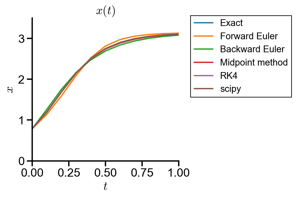
(a) Solve the ODE using backward Euler, forward Euler, midpoint method, RK4 method, and scipy.integrate.solve_ivp() from $t\in [0,1]$ with $\mathrm{\Delta }t=0.05$.

(b) Compare the solution of each method with the analytical solution.

import numpy as np
import matplotlib.pyplot as plt
import scipy
from scipy import optimize, integrate

# define the ode and analytic soln
dxdt = lambda t, x : 5*np.sin(x)
x_exact = lambda t : 2*np.arctan(np.exp(5*t) / (1 + np.sqrt(2)))

# define time steps
dt = 0.1
t_initial = 0
t_final = 1
t = np.arange(t_initial, t_final+dt/2, dt)
t_len = len(t)

# forward euler
x_forward = np.zeros(t_len)
x_forward[0] = np.pi/4

for i in range(t_len - 1):
    x_forward[i+1] = x_forward[i] + dxdt(t[i], x_forward[i])*dt

# backward euler
x_backward = np.zeros(t_len)
x_backward[0] = np.pi/4

for i in range(t_len - 1):
    g = lambda y : y - x_backward[i] - dxdt(t[i+1], y)*dt
    x_backward[i+1] = scipy.optimize.root(g, x_backward[i]).x

# midpoint method
x_midpoint = np.zeros(t_len)
x_midpoint[0] = np.pi/4

for i in range(t_len - 1):
    k1 = dxdt(t[i], x_midpoint[i])
    k2 = dxdt(t[i], x_midpoint[i] + k1*dt/2)
    x_midpoint[i+1] = x_midpoint[i] + k2*dt

# rk4 method
x_rk4 = np.zeros(t_len)
x_rk4[0] = np.pi/4

for i in range(t_len - 1):
    k1 = dxdt(t[i], x_rk4[i])
    k2 = dxdt(t[i], x_rk4[i] + k1*dt/2)
    k3 = dxdt(t[i], x_rk4[i] + k2*dt/2)
    k4 = dxdt(t[i], x_rk4[i] + k3*dt)
    x_rk4[i+1] = x_rk4[i] + (k1 + 2*k2 + 2*k3 + k4)*dt/6

# scipy.integrate.solve_ivp()
x_scipy = np.zeros(t_len)
x_scipy[0] = np.pi/4

x_scipy = scipy.integrate.solve_ivp(dxdt, [t[0], t[-1]], [t[0], x_scipy[0]], t_eval=t).y[1]

# plot settings
%config InlineBackend.figure_format = 'retina'
%matplotlib inline

plt.rcParams.update({
    'font.family': 'Arial',  # Times New Roman, Calibri
    'font.weight': 'normal',
    'mathtext.fontset': 'cm',
    'font.size': 18,
    
    'lines.linewidth': 2,
    
    'axes.linewidth': 2,
    'axes.spines.top': False,
    'axes.spines.right': False,
    'axes.titleweight': 'bold',
    'axes.titlesize': 18,
    'axes.labelweight': 'bold',
    
    'xtick.major.size': 8,
    'xtick.major.width': 2,
    'ytick.major.size': 8,
    'ytick.major.width': 2,
    
    'figure.dpi': 80,
    
    'legend.framealpha': 1, 
    'legend.edgecolor': 'black',
    'legend.fancybox': False,
    'legend.fontsize': 14
})

fig, ax = plt.subplots(figsize=(4, 4))
ax.plot(t, x_exact(t), label='Exact')
ax.plot(t, x_forward, label='Forward Euler')
ax.plot(t, x_backward, label='Backward Euler')
ax.plot(t, x_midpoint, label='Midpoint method')
ax.plot(t, x_rk4, label='RK4')
ax.plot(t, x_scipy, label='scipy')
ax.set_xlabel('$t$')
ax.set_ylabel('$x$')
ax.set_title('$x(t)$')
ax.set_xlim(t_initial, t_final)
ax.set_ylim(0, 3.5)
ax.legend(loc='upper left', bbox_to_anchor=(1.05, 1.05))

<matplotlib.legend.Legend at 0x1a9ef5d2248>

fig, ax = plt.subplots(figsize=(4, 4))
ax.plot(t, x_exact(t), label='Analytic', color='black')
ax.plot(t, x_forward, label='Forward Euler')
ax.plot(t, x_backward, label='Backward Euler')
ax.plot(t, x_midpoint, label='Midpoint method')
ax.plot(t, x_rk4, '-.', label='RK4')
ax.plot(t, x_scipy, '--', label='scipy')
ax.set_xlabel('$t$')
ax.set_ylabel('$x$')
ax.set_title('$x(t)$')
ax.set_xlim(0.5, 0.75)
ax.set_ylim(2.7, 3.1)
ax.legend(loc='upper left', bbox_to_anchor=(1.05, 1.05))

<matplotlib.legend.Legend at 0x1a9f1759648>

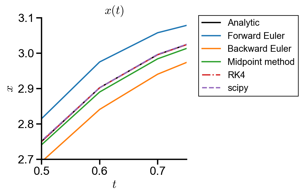
▲ The figure above shows the accuracy of each method. The RK4 and scipy solution agrees exactly with the analytic solution, having a fourth order error. The midpoint method is second closest to the analytic solution, having a second order error. Forward and backward Euler have the largest error, having a first order error.