Solving Higher-Order ODEs

Teng-Jui Lin

Content adapted from UW AMATH 301, Beginning Scientific Computing, in Spring 2020.

• Solving higher-order ODEs (systems of first-order ODEs)

  • Forward Euler

  • Backward Euler

• scipy implementation

  • Solving systems of first-order ODEs by scipy.integrate.solve_ivp()

Solving higher-order ODEs (system of ODEs)

A higher-order ODE can always be written as a system of first-order ODEs. We can then solve the first-order ODE system using forward Euler, backward Euler, or scipy.integrate.solve_ivp().

Forward Euler

Forward Euler for linear system has a similar form of

$$\begin{array}{r}\begin{array}{rl}{\mathbf{x}}_{\mathbf{k}\mathbf{+}\mathbf{1}}& ={\mathbf{x}}_{\mathbf{k}}+\mathrm{\Delta }t{\mathbf{Ax}}_{\mathbf{k}}\\ & =(\mathbf{I}+\mathrm{\Delta }t\mathbf{A}){\mathbf{x}}_{\mathbf{k}}\end{array}\end{array}$$

The method is stable when all of the absolute value of eigenvalues of $\mathbf{I}+\mathrm{\Delta }t\mathbf{A}$ are less than 1: $|\lambda |<1$.

Backward Euler

Backward Euler for linear system has a similar form of

$${\mathbf{x}}_{\mathbf{k}\mathbf{+}\mathbf{1}}\mathbf{=}{\mathbf{x}}_{\mathbf{k}}+\mathrm{\Delta }t{\mathbf{Ax}}_{\mathbf{k}\mathbf{+}\mathbf{1}}$$

that can be implemented as

$$(\mathbf{I}-\mathrm{\Delta }t\mathbf{A}){\mathbf{x}}_{\mathbf{k}\mathbf{+}\mathbf{1}}={\mathbf{x}}_{\mathbf{k}}$$

which can be implemented with LU decomposition. The method is stable when all of the absolute value of eigenvalues of $(\mathbf{I}-\mathrm{\Delta }t\mathbf{A}{)}^{-1}$ are less than 1: $|\lambda |<1$.

Implementation

Problem Statement. Linear pendulum.

The motion of a linear pendulum at small angles can be described by the linear second-order ODE

$$\ddot{\theta }=-{\displaystyle \frac{g}{L}}\theta$$

where $\theta$ is the angle of deflection of the pendulum from the vertical. Given physical parameters $L=1\mathrm{m}$ and $g=9.8\mathrm{m}/{\mathrm{s}}^2$.

The second-order ODE can be converted to a system of two first-order ODEs

$$\begin{array}{r}\{\begin{array}{l}\dot{\theta }=\omega \\ \dot{\omega }=-{\displaystyle \frac{g}{L}}\theta \end{array}\end{array}$$

which is equivalent to

$$\dot{\mathbf{x}}\mathbf{=}\mathbf{Ax}$$

where

$$\begin{array}{r}\mathbf{x}=\left[\begin{array}{c}\theta \\ \omega \end{array}\right],\mathbf{A}=\left[\begin{array}{cc}0& 1\\ -{\displaystyle \frac{g}{L}}& 0\end{array}\right]\end{array}$$

For the initial conditions $\theta (0)=0,\dot{\theta }(0)=\omega (0)=0.5$, we will solve the system of ODEs over $t\in [0,10]\mathrm{s}$ using numerical methods, then we compare the results with it analytical solution of

$$\begin{array}{r}\mathbf{x}(t)=\left[\begin{array}{c}\theta (t)\\ \omega (t)\end{array}\right]=\left[\begin{array}{c}0.5\sqrt{\frac{L}{g}}\sin (\sqrt{\frac{g}{L}}t)\\ 0.5\cos (\sqrt{\frac{g}{L}}t)\end{array}\right].\end{array}$$

(a) Use forward Euler for linear system with $\mathrm{\Delta }t=0.005\mathrm{s}$ to solve the system. Determine the stability of the method and compare the error at final time with the analytical solution.

(b) Use backward Euler for linear system with $\mathrm{\Delta }t=0.005\mathrm{s}$ using LU decomposition. Determine the stability of the method and compare the error at final time with the analytical solution.

(c) Use scipy.integrate.solve_ivp() to solve the system. Compare the error at final time with the analytical solution.

Forward Euler

import numpy as np
import matplotlib.pyplot as plt
import scipy
from scipy import integrate

# define physical constants
g = 9.8
l = 1

# define time array
t_initial = 0
t_final = 10
dt = 0.005
t = np.arange(t_initial, t_final+dt/2, dt)
t_len = len(t)

# define matrix and initial conditions
A = np.array([[0, 1], [-g/l, 0]])
x0 = np.array([0, 0.5])
x = np.zeros((2, t_len))
x[:, 0] = x0

# forward euler of linear system
for i in range(t_len - 1):
    x[:, i+1] = x[:, i] + dt*A@x[:, i]

# compare with analytical soln
x_exact = lambda t : np.array([0.5 * np.sqrt(l/g) *np.sin(t*np.sqrt(g/l)),
                               0.5 * np.cos(t*np.sqrt(g/l))])
x_error = np.linalg.norm(x[:, -1] - x_exact(t_final))
print(f'Error = {x_error :.2f}')

Error = 0.14

# assess stability
stability_matrix = np.eye(len(A)) + dt*A
abs_eig = abs(np.linalg.eig(stability_matrix)[0])
if max(abs_eig) > 1:
    print(f'Unstable with |lambda_max| = {max(abs_eig) :.4f}')
else:
    print(f'Stable with |lambda_max| = {max(abs_eig) :.4f}')

Unstable with |lambda_max| = 1.0001

# plot settings
%config InlineBackend.figure_format = 'retina'
%matplotlib inline

plt.rcParams.update({
    'font.family': 'Arial',  # Times New Roman, Calibri
    'font.weight': 'normal',
    'mathtext.fontset': 'cm',
    'font.size': 18,
    
    'lines.linewidth': 2,
    
    'axes.linewidth': 2,
    'axes.spines.top': False,
    'axes.spines.right': False,
    'axes.titleweight': 'bold',
    'axes.titlesize': 18,
    'axes.labelweight': 'bold',
    
    'xtick.major.size': 8,
    'xtick.major.width': 2,
    'ytick.major.size': 8,
    'ytick.major.width': 2,
    
    'figure.dpi': 80,
    
    'legend.framealpha': 1, 
    'legend.edgecolor': 'black',
    'legend.fancybox': False,
    'legend.fontsize': 14
})

fig, ax = plt.subplots(figsize=(4, 4))
ax.plot(t, x_exact(t)[0], '--', label='Analytic')
ax.plot(t, x[0], label='Forward Euler')
ax.set_xlabel('$t \ [\mathrm{s}]$')
ax.set_ylabel('$\\theta \ [\mathrm{rad}]$')
ax.set_title('$\\theta(t)$')
ax.set_xlim(t_initial, t_final)
ax.set_ylim(-0.3, 0.3)
ax.legend(loc='upper left', bbox_to_anchor=(1.05, 1.05))

<matplotlib.legend.Legend at 0x2a5d7de2c88>

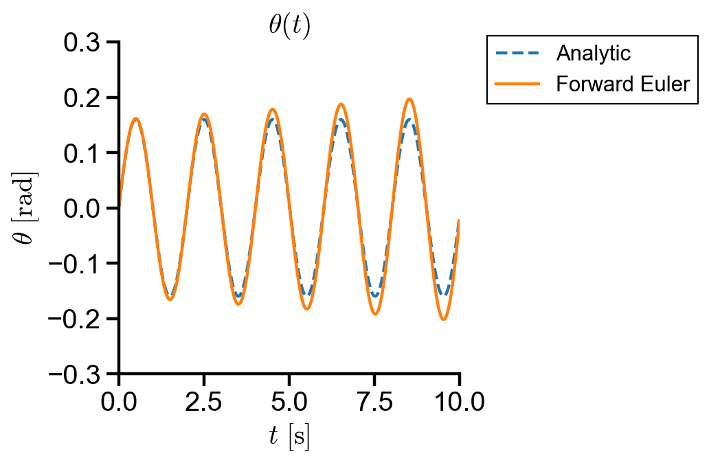
▲ Forward Euler has first order error and the amplitude grows over time compared to the analytic solution.

Backward Euler

# define physical constants
g = 9.8
l = 1

# define time array
t_initial = 0
t_final = 10
dt = 0.005
t = np.arange(t_initial, t_final+dt/2, dt)
t_len = len(t)

# define matrix and initial conditions
A = np.array([[0, 1], [-g/l, 0]])
x0 = np.array([0, 0.5])
x = np.zeros((2, t_len))
x[:, 0] = x0

P, L, U = scipy.linalg.lu(np.eye(len(A)) - dt*A)

# backward euler of linear system
for i in range(t_len - 1):
    y = np.linalg.solve(L, P@x[:, i])
    x[:, i+1] = np.linalg.solve(U, y)

# compare with analytical soln
x_exact = lambda t : np.array([0.5 * np.sqrt(l/g) *np.sin(t*np.sqrt(g/l)),
                               0.5 * np.cos(t*np.sqrt(g/l))])
x_error = np.linalg.norm(x[:, -1] - x_exact(t_final))
print(f'Error = {x_error :.2f}')

Error = 0.11

# assess stability
stability_matrix = np.linalg.inv(np.eye(len(A)) - dt*A)
abs_eig = abs(np.linalg.eig(stability_matrix)[0])
if max(abs_eig) > 1:
    print(f'Unstable with |lambda_max| = {max(abs_eig) :.4f}')
else:
    print(f'Stable with |lambda_max| = {max(abs_eig) :.4f}')

Stable with |lambda_max| = 0.9999

fig, ax = plt.subplots(figsize=(4, 4))
ax.plot(t, x_exact(t)[0], '--', label='Analytic')
ax.plot(t, x[0], label='Backward Euler')
ax.set_xlabel('$t \ [\mathrm{s}]$')
ax.set_ylabel('$\\theta \ [\mathrm{rad}]$')
ax.set_title('$\\theta(t)$')
ax.set_xlim(t_initial, t_final)
ax.set_ylim(-0.3, 0.3)
ax.legend(loc='upper left', bbox_to_anchor=(1.05, 1.05))

<matplotlib.legend.Legend at 0x2a5d80d4108>

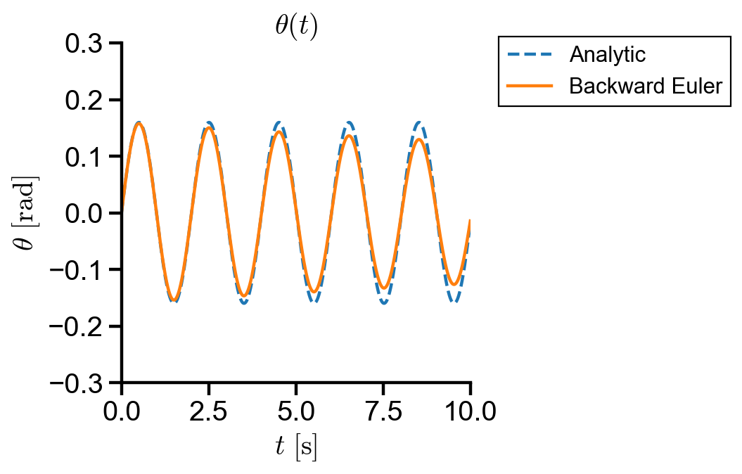
▲ Backward Euler has first order error and the amplitude decays over time compared to the analytic solution.

scipy.integrate.solve_ivp()

# define physical constants
g = 9.8
l = 1

# define time array
t_initial = 0
t_final = 10
dt = 0.005
t = np.arange(t_initial, t_final+dt/2, dt)
t_len = len(t)

# define initial conditions
x0 = np.array([0, 0.5])

# define ode system
dtheta_dt = lambda theta, omega : omega
domega_dt = lambda theta, omega: -g/l*theta
ode_syst = lambda t, z : np.array([dtheta_dt(*z), domega_dt(*z)])

# solve ode system
scipy_soln = scipy.integrate.solve_ivp(ode_syst, [t_initial, t_final], x0, t_eval=t).y

# compare with analytical soln
x_exact = lambda t : np.array([0.5 * np.sqrt(l/g) *np.sin(t*np.sqrt(g/l)),
                               0.5 * np.cos(t*np.sqrt(g/l))])
x_error = np.linalg.norm(scipy_soln[:, -1] - x_exact(t_final))
print(f'Error = {x_error :.4f}')

Error = 0.0015

fig, ax = plt.subplots(figsize=(4, 4))
ax.plot(t, x_exact(t)[0], '--', label='Analytic')
ax.plot(t, scipy_soln[0], label='scipy')
ax.set_xlabel('$t \ [\mathrm{s}]$')
ax.set_ylabel('$\\theta \ [\mathrm{rad}]$')
ax.set_title('$\\theta(t)$')
ax.set_xlim(t_initial, t_final)
ax.set_ylim(-0.3, 0.3)
ax.legend(loc='upper left', bbox_to_anchor=(1.05, 1.05))

<matplotlib.legend.Legend at 0x2a5b61a6ec8>

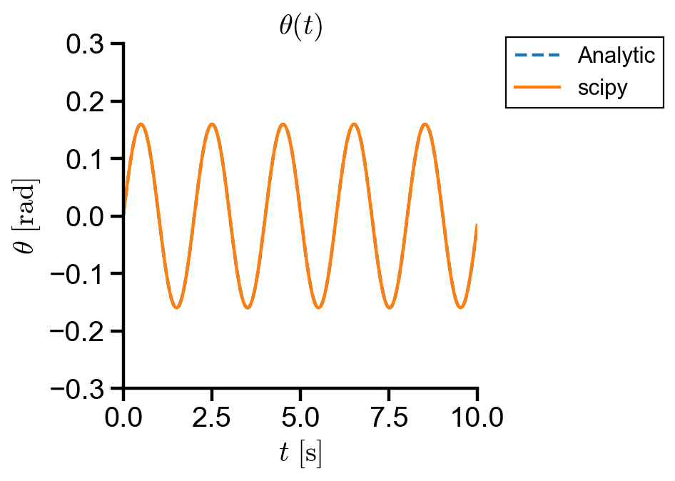
▲ The scipy implementation has fourth order error, agreeing with the analytic solution.